
Evan Trock
Data Section
- This data shows observations about a sample of homes that have been built over a long span of time(1852-2008), It shows different types of add-ons for a house, square footage, type of street and information about the sale of the property but most of all, the sales price
- 1941 Observations in this data set
- Year Sold Ranging from 2006-2008
- No Duplicate Parcels
- Certain Variables have missing values including: v_Mas_Vnr_Area(Missing 18) v_BsmtFin_SF_1, v_BsmtFin_SF_2(Both missing 1), and v_Lot_Frontage(Missing 321)
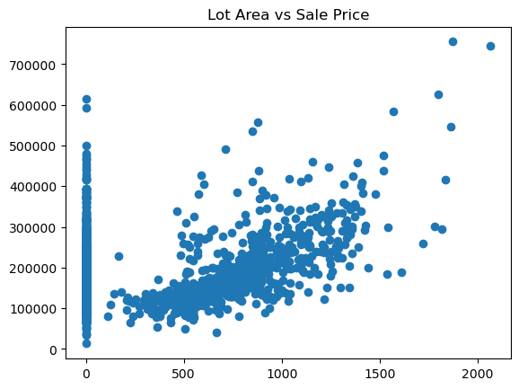
- A couple of outliers in the Sales price category: I determined it is over 60000 for smaller houses, and lot size with lower prices looks to be over 70000.
- Data comes from a City called Ames in Iowa
- Continous variables include but are not limited to many area variables: Lot size, price, pool_area, porch area, as well as street front property size Notes: Strong correlation between price and these variables, not as big as expected in lot size, but large correlation in square feet of 1st and 2nd floor
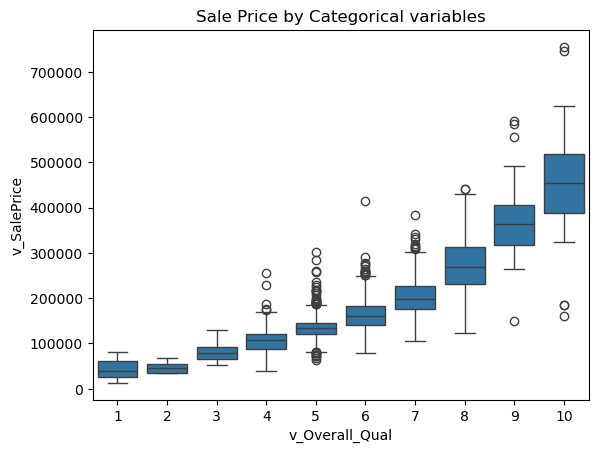
- Categorical Variables include types and styles like roof type and style, neighborhood, lot configuration and type of road access Notes: Strong correlation between price and the condition of the house at sale, showing new houses go for more, and variables like Overall quality
- Discrete Variables include number of bedrooms, kitchen, bathrooms and so on
import pandas as pd
from statsmodels.formula.api import ols as sm_ols
import numpy as np
import seaborn as sns
from statsmodels.iolib.summary2 import summary_col # nicer tables
import matplotlib.pyplot as plt

data = pd.read_csv('input_data2/housing_train.csv')
data.describe()
| v_MS_SubClass | v_Lot_Frontage | v_Lot_Area | v_Overall_Qual | v_Overall_Cond | v_Year_Built | v_Year_Remod/Add | v_Mas_Vnr_Area | v_BsmtFin_SF_1 | v_BsmtFin_SF_2 | ... | v_Wood_Deck_SF | v_Open_Porch_SF | v_Enclosed_Porch | v_3Ssn_Porch | v_Screen_Porch | v_Pool_Area | v_Misc_Val | v_Mo_Sold | v_Yr_Sold | v_SalePrice | |
|---|---|---|---|---|---|---|---|---|---|---|---|---|---|---|---|---|---|---|---|---|---|
| count | 1941.000000 | 1620.000000 | 1941.000000 | 1941.000000 | 1941.000000 | 1941.000000 | 1941.000000 | 1923.000000 | 1940.000000 | 1940.000000 | ... | 1941.000000 | 1941.000000 | 1941.000000 | 1941.000000 | 1941.000000 | 1941.000000 | 1941.000000 | 1941.000000 | 1941.000000 | 1941.000000 |
| mean | 58.088614 | 69.301235 | 10284.770222 | 6.113344 | 5.568264 | 1971.321999 | 1984.073158 | 104.846074 | 436.986598 | 49.247938 | ... | 92.458011 | 49.157135 | 22.947965 | 2.249871 | 16.249871 | 3.386399 | 52.553838 | 6.431221 | 2006.998454 | 182033.238022 |
| std | 42.946015 | 23.978101 | 7832.295527 | 1.401594 | 1.087465 | 30.209933 | 20.837338 | 184.982611 | 457.815715 | 169.555232 | ... | 127.020523 | 70.296277 | 65.249307 | 22.416832 | 56.748086 | 43.695267 | 616.064459 | 2.745199 | 0.801736 | 80407.100395 |
| min | 20.000000 | 21.000000 | 1470.000000 | 1.000000 | 1.000000 | 1872.000000 | 1950.000000 | 0.000000 | 0.000000 | 0.000000 | ... | 0.000000 | 0.000000 | 0.000000 | 0.000000 | 0.000000 | 0.000000 | 0.000000 | 1.000000 | 2006.000000 | 13100.000000 |
| 25% | 20.000000 | 58.000000 | 7420.000000 | 5.000000 | 5.000000 | 1953.000000 | 1965.000000 | 0.000000 | 0.000000 | 0.000000 | ... | 0.000000 | 0.000000 | 0.000000 | 0.000000 | 0.000000 | 0.000000 | 0.000000 | 5.000000 | 2006.000000 | 130000.000000 |
| 50% | 50.000000 | 68.000000 | 9450.000000 | 6.000000 | 5.000000 | 1973.000000 | 1993.000000 | 0.000000 | 361.500000 | 0.000000 | ... | 0.000000 | 28.000000 | 0.000000 | 0.000000 | 0.000000 | 0.000000 | 0.000000 | 6.000000 | 2007.000000 | 161900.000000 |
| 75% | 70.000000 | 80.000000 | 11631.000000 | 7.000000 | 6.000000 | 2001.000000 | 2004.000000 | 168.000000 | 735.250000 | 0.000000 | ... | 168.000000 | 72.000000 | 0.000000 | 0.000000 | 0.000000 | 0.000000 | 0.000000 | 8.000000 | 2008.000000 | 215000.000000 |
| max | 190.000000 | 313.000000 | 164660.000000 | 10.000000 | 9.000000 | 2008.000000 | 2009.000000 | 1600.000000 | 5644.000000 | 1474.000000 | ... | 1424.000000 | 742.000000 | 1012.000000 | 407.000000 | 576.000000 | 800.000000 | 17000.000000 | 12.000000 | 2008.000000 | 755000.000000 |
8 rows × 37 columns
# graph continuous data
plt.plot(data['v_2nd_Flr_SF'], data['v_SalePrice'], 'o')
plt.title('Lot Area vs Sale Price')
plt.show()
#Graph categorical data
sns.boxplot(x='v_Overall_Qual', y='v_SalePrice', data=data)
plt.title('Sale Price by Categorical variables')
Text(0.5, 1.0, 'Sale Price by Categorical variables')
print('Regression Results:')
reg1 = sm_ols('v_SalePrice ~  v_Lot_Area ', data=data).fit()
logLotArea = np.log(data['v_Lot_Area'])
reg2 = sm_ols('v_SalePrice ~  logLotArea ', data=data).fit()
logSalePrice = np.log(data['v_SalePrice'])
reg3 = sm_ols('logSalePrice ~  v_Lot_Area ', data=data).fit()
reg4 = sm_ols('logSalePrice ~  logLotArea ', data=data).fit()
reg5 = sm_ols('logSalePrice ~  v_Yr_Sold ', data=data).fit()
data['v_Yr_Sold_2007'] = (data['v_Yr_Sold'] == 2007).astype(int)
data['v_Yr_Sold_2008'] = (data['v_Yr_Sold'] == 2008).astype(int)
reg6 = sm_ols('logSalePrice ~  v_Yr_Sold_2007 + v_Yr_Sold_2008 ', data=data).fit()
log1stFlr = np.log(data['v_1st_Flr_SF'])
logQual = np.log(data['v_Overall_Qual'])
reg7 = sm_ols('logSalePrice ~  v_Kitchen_Qual + log1stFlr + v_Functional + logQual + v_Gr_Liv_Area ', data=data).fit()

print(summary_col(results=[reg1,reg2,reg3,reg4,reg5,reg6,reg7], # list the result obj here
                  float_format='%0.2f',
                  stars = True, # stars are easy way to see if anything is statistically significant
                  model_names=['No Log','Log Area','No AreaLog','Both Log','Yr Sold','2007+2008',
                               '5 Variable Model'],
                  )
     )
Regression Results:

======================================================================================================
                        No Log       Log Area   No AreaLog Both Log Yr Sold 2007+2008 5 Variable Model
------------------------------------------------------------------------------------------------------
Intercept            154789.55*** -327915.80*** 11.89***   9.41***  22.29   12.02***  8.48***
                     (2911.59)    (30221.35)    (0.01)     (0.15)   (22.94) (0.02)    (0.11)
v_Lot_Area           2.65***                    0.00***
                     (0.23)                     (0.00)
logLotArea                        56028.17***              0.29***
                                  (3315.14)                (0.02)
v_Yr_Sold                                                           -0.01
                                                                    (0.01)
v_Yr_Sold_2007                                                              0.03
                                                                            (0.02)
v_Yr_Sold_2008                                                              -0.01
                                                                            (0.02)
v_Kitchen_Qual[T.Fa]                                                                  -0.31***
                                                                                      (0.03)
v_Kitchen_Qual[T.Gd]                                                                  -0.10***
                                                                                      (0.02)
v_Kitchen_Qual[T.TA]                                                                  -0.23***
                                                                                      (0.02)
v_Functional[T.Maj2]                                                                  -0.13
                                                                                      (0.08)
v_Functional[T.Min1]                                                                  0.19***
                                                                                      (0.05)
v_Functional[T.Min2]                                                                  0.16***
                                                                                      (0.05)
v_Functional[T.Mod]                                                                   0.20***
                                                                                      (0.06)
v_Functional[T.Sal]                                                                   -0.61***
                                                                                      (0.13)
v_Functional[T.Sev]                                                                   -0.24
                                                                                      (0.18)
v_Functional[T.Typ]                                                                   0.24***
                                                                                      (0.05)
log1stFlr                                                                             0.27***
                                                                                      (0.01)
logQual                                                                               0.69***
                                                                                      (0.02)
v_Gr_Liv_Area                                                                         0.00***
                                                                                      (0.00)
R-squared            0.07         0.13          0.06       0.13     0.00    0.00      0.82
R-squared Adj.       0.07         0.13          0.06       0.13     -0.00   0.00      0.82
======================================================================================================
Standard errors in parentheses.
* p<.1, ** p<.05, ***p<.01
#3
print(summary_col(results=[reg5, reg6 ],
                  float_format='%0.6f',
                  stars=True,
                  model_names=['Reg 5', 'reg6']
                 )
     )
=======================================
                  Reg 5        reg6
---------------------------------------
Intercept      22.293213   12.022869***
               (22.936825) (0.016136)
v_Yr_Sold      -0.005114
               (0.011428)
v_Yr_Sold_2007             0.025590
                           (0.022246)
v_Yr_Sold_2008             -0.010282
                           (0.022848)
R-squared      0.000103    0.001436
R-squared Adj. -0.000412   0.000406
=======================================
Standard errors in parentheses.
* p<.1, ** p<.05, ***p<.01
- Regression outputs and R-Squared Shown above
- $\beta_1$ = 56028.17. This means that if the lot area increases by 1%, the predicted sale price increases by approximately $560.28
- $\beta_1$ = 0.000013 it’s a very small positive number, it means that for each additional square foot of lot area, the sale price increases by a .013 cents
- Looking at R squared first, Model 2 and 4 have a leg up at .13. To distinguish them, the elasticity is more interpretable for model 2 than 4 so I beleive model 2 represents the data the best.
- $\beta_1$ = -0.01. This means that, holding the effects of sales in 2007 and 2008 constant, each additional year of sale is associated with a decrease of $0.01 in sale price.
- $\alpha$ = 12.02. This represents the predicted sale price when v_Yr_Sold, v_Yr_Sold_2007, and v_Yr_Sold_2008 are all zero. In the context of this model, it’s the baseline sale price for years other than 2007 or 2008
- $\beta_1$ = .03 : This means that, holding the year of sale and the effect of 2008 constant, sales in 2007 were associated with a 0.03 increase in sale price.
- The indicator variables in model 6 provide more explanatory power, leading to a higher R-squared, even though the overall R-squared values are still very low, with the data split between 2 years for model 6
- I used logSalePrice and v_1st_Flr_SF, measuring the 1st floor square footage versus the sale price
- 0.82 is the R-Squared from my 5 variable model
- Although it could be used for a predictive regression to predicting house prices in the 2007/2008 period, I don’t think that it necessarily should as the low R squared value of .001436 suggests that it is more of a correlation rather than causation and the 2 variables are not very related.
- Similar to number 11, model 5 has a very small R-Squared value at .000103 and should not be used for predictive analysis.