Machine Learning Practice

Objectives:

Preprocesses realistic data (multiple variable types) in a pipeline that handles each variable type
Estimates a model using CV
Hypertunes a model on a CV folds within training sample
Finally, evaluate its performance in the test sample

Let’s start by loading the data

import pandas as pd
import numpy as np
from sklearn.model_selection import train_test_split

# load data and split off X and y
housing = pd.read_csv('input_data2/housing_train.csv')
y = np.log(housing.v_SalePrice)
housing = housing.drop('v_SalePrice',axis=1)

Per the recommendations in the sk-learn documentation, what that means is we need to put random_state=rng inside every function in this file that accepts “random_state” as an argument.

# create test set for use later - notice the (random_state=rng)
rng = np.random.RandomState(0)
X_train, X_test, y_train, y_test = train_test_split(housing, y, random_state=rng)

Part 1: Preprocessing the data

from sklearn.compose import make_column_transformer, make_column_selector
from sklearn.pipeline import make_pipeline
from sklearn.impute import SimpleImputer
from sklearn.preprocessing import StandardScaler, OneHotEncoder

# Define pipelines for numerical and categorical data
numer_pipe = make_pipeline(
    SimpleImputer(strategy="mean"),
    StandardScaler())
cat_pipe = make_pipeline(
    OneHotEncoder(handle_unknown="ignore"))
# Combine the pipelines into a single preprocessing pipeline
preproc_pipe = make_column_transformer(
    (numer_pipe, make_column_selector(dtype_include=["int64", "float64"])),
    (cat_pipe, ["v_Lot_Config"]),
    remainder="drop"  # Drop all other variables
)
# Fit the pipeline and transform X_train
preproc_pipe.fit(X_train)

# Get feature names from the pipeline
numerical_features = preproc_pipe.named_transformers_['pipeline-1'].get_feature_names_out()
categorical_features = preproc_pipe.named_transformers_['pipeline-2'].get_feature_names_out(["v_Lot_Config"])
all_features = list(numerical_features) + list(categorical_features)

# Transform the data and create a DataFrame with proper column names
X_train_preprocessed = preproc_pipe.transform(X_train)
X_train_preprocessed_df = pd.DataFrame(
    X_train_preprocessed.toarray() if hasattr(X_train_preprocessed, "toarray") else X_train_preprocessed,
    columns=all_features
)
# Output the number of columns
print(f"Number of columns in preprocessed data: {X_train_preprocessed_df.shape[1]}")
X_train_preprocessed_df.describe().round(2)

Number of columns in preprocessed data: 41

	v_MS_SubClass	v_Lot_Frontage	v_Lot_Area	v_Overall_Qual	v_Overall_Cond	v_Year_Built	v_Year_Remod/Add	v_Mas_Vnr_Area	v_BsmtFin_SF_1	v_BsmtFin_SF_2	...	v_Screen_Porch	v_Pool_Area	v_Misc_Val	v_Mo_Sold	v_Yr_Sold	v_Lot_Config_Corner	v_Lot_Config_CulDSac	v_Lot_Config_FR2	v_Lot_Config_FR3	v_Lot_Config_Inside
count	1455.00	1455.00	1455.00	1455.00	1455.00	1455.00	1455.00	1455.00	1455.00	1455.00	...	1455.00	1455.00	1455.00	1455.00	1455.00	1455.00	1455.00	1455.00	1455.00	1455.00
mean	0.00	0.00	0.00	0.00	0.00	-0.00	0.00	0.00	0.00	0.00	...	-0.00	-0.00	-0.00	-0.00	-0.00	0.18	0.06	0.02	0.01	0.73
std	1.00	1.00	1.00	1.00	1.00	1.00	1.00	1.00	1.00	1.00	...	1.00	1.00	1.00	1.00	1.00	0.38	0.24	0.15	0.08	0.44
min	-0.89	-2.20	-1.17	-3.70	-4.30	-3.08	-1.63	-0.57	-0.96	-0.29	...	-0.29	-0.08	-0.09	-2.03	-1.24	0.00	0.00	0.00	0.00	0.00
25%	-0.89	-0.43	-0.39	-0.81	-0.53	-0.62	-0.91	-0.57	-0.96	-0.29	...	-0.29	-0.08	-0.09	-0.55	-1.24	0.00	0.00	0.00	0.00	0.00
50%	-0.20	0.00	-0.11	-0.09	-0.53	0.05	0.43	-0.57	-0.16	-0.29	...	-0.29	-0.08	-0.09	-0.18	0.00	0.00	0.00	0.00	0.00	1.00
75%	0.26	0.39	0.19	0.64	0.41	0.98	0.96	0.33	0.65	-0.29	...	-0.29	-0.08	-0.09	0.56	1.25	0.00	0.00	0.00	0.00	1.00
max	3.03	11.07	20.68	2.80	3.24	1.22	1.20	7.87	11.20	8.29	...	9.69	17.05	24.19	2.04	1.25	1.00	1.00	1.00	1.00	1.00

8 rows × 41 columns

Part 2: Estimating one model

from sklearn.linear_model import LassoCV
from sklearn.pipeline import Pipeline
from sklearn.model_selection import cross_val_score, KFold
# Define the LassoCV model
lasso_cv_model = LassoCV(cv=10, random_state=rng)
# Create a pipeline combining the preprocessor and the LassoCV model
model_pipeline = Pipeline([
    ('preprocessor', preproc_pipe), ('lasso_cv', lasso_cv_model)
])
# Perform 10-fold cross-validation with R^2 scoring
cv = KFold(n_splits=10, shuffle=True, random_state=rng)
cv_scores = cross_val_score(model_pipeline, X_train, y_train, cv=cv, scoring='r2')
mean_score = cv_scores.mean()
print(f"1. Mean Score: {mean_score:.5f}")

1. Mean Score: 0.83437

#b
lasso_cv_model = LassoCV(cv=10, random_state=rng)
# Fit the pipeline to the training data
model_pipeline.fit(X_train, y_train)

optimal_alpha = model_pipeline.named_steps['lasso_cv'].alpha_
print(f"2.1) Optimal alpha: {optimal_alpha:.5f}")
r2_score_train = model_pipeline.score(X_train, y_train)
print(f"2.2) R^2 score on test set: {r2_score_train:.5f}")
coefficients = model_pipeline.named_steps['lasso_cv'].coef_
nonZeroNumber = (coefficients != 0).sum()
print(f"2.3) # of Variables Selected: {nonZeroNumber}")

coefficients = model_pipeline.named_steps['lasso_cv'].coef_
feature_names = all_features  
coef_df = pd.DataFrame({
    'Feature': feature_names, 'Coefficient': coefficients
})
non_zero = coef_df[coef_df['Coefficient'] != 0]
top5 = non_zero.nlargest(5, 'Coefficient')
print(f"2.4) Top 5 non-zero coefficients:")
print(top5)
bot5 = non_zero.nsmallest(5, 'Coefficient')
print(f"2.5) Bottotm 5 non-zero coefficients:")
print(bot5)
r2_score_test = model_pipeline.score(X_test, y_test)
print(f"2.6) R^2 score on test set: {r2_score_test:.5f}")

1) Optimal alpha: 0.00802
2) R^2 score on test set: 0.86264
3) # of Variables Selected: 21
4) Top 5 non-zero coefficients:
           Feature  Coefficient
 v_Overall_Qual     0.134599
 v_Gr_Liv_Area     0.098313
   v_Year_Built     0.065831
 v_Garage_Cars     0.047635
 v_Overall_Cond     0.035216
5) Bottotm 5 non-zero coefficients:
            Feature  Coefficient
   v_MS_SubClass    -0.020093
     v_Misc_Val    -0.017537
v_Kitchen_AbvGr    -0.003737
    v_Pool_Area    -0.002016
v_Bedroom_AbvGr     0.003556
6) R^2 score on test set: 0.86503

Part 3: Optimizing and estimating your own model

#1. 
from sklearn.preprocessing import PolynomialFeatures
from sklearn.decomposition import PCA
from sklearn.ensemble import HistGradientBoostingRegressor

# Preprocessing
numer_pipe = Pipeline([
    ('imputer', SimpleImputer(strategy='mean')), ('scaler', StandardScaler()),
    ('poly', PolynomialFeatures(degree=2, include_bias=False))  
])
cat_pipe = Pipeline([('imputer', SimpleImputer(strategy='most_frequent')), ('onehot', OneHotEncoder(handle_unknown='ignore'))])
preproc_pipe = make_column_transformer(
    (numer_pipe, make_column_selector(dtype_include=['int64', 'float64'])),
    (cat_pipe, make_column_selector(dtype_include=['object'])),
    remainder='drop'
)
#Full Pipeline
pipeline = Pipeline([
    ("preprocessor", preproc_pipe),
    ("feature_select", PCA(n_components=20, random_state=rng)),
    ("model", HistGradientBoostingRegressor(random_state=rng))
])
print("Output 1")
pipeline

Output 1

from sklearn.model_selection import GridSearchCV
# Define grid
param_grid = {
    "feature_select__n_components": [ 60, 70, 80, 90, 100],
    "model__max_leaf_nodes": [10, 20, 30, 50, 70]
}
grid_search = GridSearchCV(estimator = pipeline, 
                           param_grid = param_grid,
                           cv = 5, 
                           scoring= 'r2',
                           n_jobs=-1,
                           return_train_score=True
                           )
grid_search.fit(X_train,y_train)
# Results
print("Best Parameters:", grid_search.best_params_)
print(f"Best CV R^2 Score: {grid_search.best_score_:.5f}")

Best Parameters: {'feature_select__n_components': 70, 'model__max_leaf_nodes': 10}
Best CV R^2 Score: 0.80113

Output 2

feature_select__n_components(PCA) sets how many principal components to keep after running PCA. This helps to optimize the performance and avoid overfitting or underfitting.

model__max_leaf_nodes (HistGradientBoostingRegressor) shows the the maximum number of leaf nodes per decision tree. Optimizing this is important to find the right complexity for each tree as more leafs is better for more complex trees whereas less leafs is better for simpler trees.

#Output 3
import matplotlib.pyplot as plt

results = grid_search.cv_results_
mean_test_scores = results['mean_test_score']
std_test_scores = results['std_test_score']
params = results['params']
# Find the index of the best model
best_index = np.argmax(mean_test_scores)
best_params = params[best_index]
# Plot 25 tests
plt.figure(figsize=(10, 6))
plt.errorbar(std_test_scores, mean_test_scores, fmt='o', label='Models', alpha=0.7)
plt.scatter(std_test_scores[best_index], mean_test_scores[best_index], color='red', s=100, label='Best Model')
# Show the red: Best Model with its parameters
plt.annotate(f"Best Model\n{best_params}", 
             (std_test_scores[best_index], mean_test_scores[best_index]),
             textcoords="offset points", xytext=(10, -20), ha='center', fontsize=10, color='red')
plt.xlabel('Standard Deviation of CV Test Scores')
plt.ylabel('Mean CV Test Scores')
plt.title('Grid Search Results: Mean vs. STD of CV Test Scores')
plt.legend()
plt.grid(True)
plt.show()

png

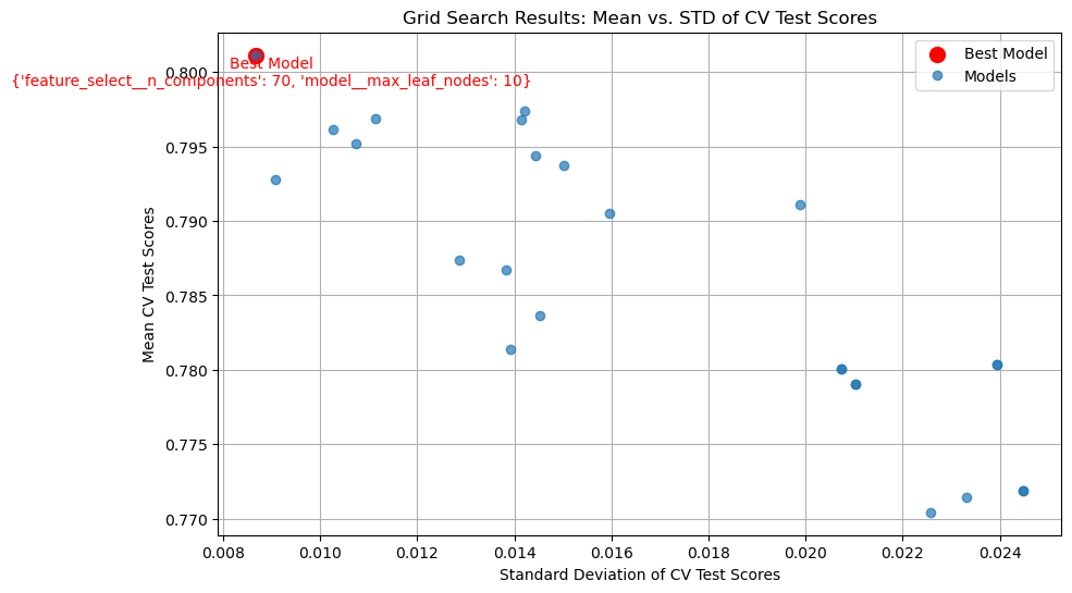
Output 4

For feature_select__n_components, I used [60, 70,80,90,100], as these values avoided over and underfitting and the eventual value was not the minimum or maximum. The same goes for model__max_leaf_nodes, although the values were different at [10, 20, 30, 50, 70].

from sklearn.metrics import r2_score

best_model = grid_search.best_estimator_
y_pred_test = best_model.predict(X_test)
test_r2 = r2_score(y_test, y_pred_test)
print(f"Output 5: Final R2 on test set: {test_r2:.5f}")

Output 5: Final R2 on test set: 0.78267